Poor robots. All around the internet are little ‘CAPTCHA’ checkboxes designed to keep them out. That terrible tickmark—“I am not a robot”—has caused many a positronic tear. Well, it’s time someone thought about the robots. I created a dedicated website for robots and harnessed the power of probability to keep humans out.

I initially built this website — and wrote an earlier version of this write-up — for CS109, an introductory probability class I took in the winter of 2021. The challenge was to make something cool that leveraged the concepts we’d learned in class. This website is what I came up with.

You can explore the website at https://robots.rmrm.io, and the source code is available at https://github.com/milesmcc/random-game. I suggest using the website at least once before reading this write-up.

Expected audience: Someone familiar with introductory probability. If that’s not you, all good — just skip over all the math stuff. You’ll hopefully still get the gist of it!

Detecting Humans

Humans are quite bad at producing random numbers, and we can use this fact to our advantage.¹ If we ask them to produce a random stream of numbers (by pressing the digit keys on their keyboard), perhaps they’ll reveal themselves by producing values that deviate from the expected distribution. Take that, humans!

Of course, this approach makes several assumptions. For example, while humans’ relative inability to produce properly-distributed random numbers is well-documented, having a keyboard in front of them may (or may not) help them do a better job. Beyond this high-level assumption, however, we will try to assume as little as possible about human behavior in constructing our model.

There are two clear ways we can identify humans through their ‘random’ values: by looking at the frequencies of the selected digits,² and by looking at the distances between the digits as they are selected.³

Primitive Frequency Analysis

When asked to produce random uniform digits, humans rarely produce an even distribution. Instead, they tend to bias towards particular values (e.g., 7) and away from others (e.g., 5).⁴ We can assess the probability of any particular frequency breakdown using a multinomial distribution where the probability of any particular digit is equally likely. The expected outcome, then, is a uniform distribution, and the probability of \(n\) uniform random variables producing \(N_0\) 0’s, \(N_1\) 1’s, etc. is:

$$\binom{n!}{N_0, N_1, … N_9} \left(\frac{1}{10}\right)^n$$

This probability is not particularly useful on its own, however. With only ten samples, the highest possible probability is \(10! * 0.1^{10}\). Instead, we are more interested in this probability in relation to others. Ideally, we could somehow employ it in computing \(P(\text{robot} \mid \text{observed})\). While on its face this resembles a straightforward application of Bayes’ rule, problems quickly arise:

$$P(\text{robot} \mid \text{observed}) = \frac{P(\text{observed} \mid \text{robot}) * P(\text{robot})}{P(\text{observed})}$$

What is \(P(\text{robot})\)? I don’t know — and I have no experimental data from which I could estimate. A similar issue exists for \(P(\text{observed})\): we know the probability of observing the sample data conditioned on uniformity, but we have no insight into the unconditioned case.

At a glance, this conundrum looks like a great place for bootstrapping some kind of \(p\)-value. Unfortunately, that approach is not much help here: it considers the sample mean and other attributes of a distribution (e.g., variance), while we are more broadly interested in goodness of fit. A human might successfully produce numbers that average to 4.5 — the expected value of our uniform distribution — but that does not mean that the distribution of those numbers is uniform. Instead, we need a true goodness of fit test.

Assessing Goodness of Fit

For the challenge, I explored and experimented with two different goodness of fit tests: the Kolmogorov-Smirnov test and the Andersen-Darling test. The Kolmogorov-Smirnov (K-S) test captures the largest deviation of the observed distribution’s CDF from the expected distribution’s CDF; the higher the value, the more confident we can be that the observed distribution isn’t drawn from a uniform random variable. Wikipedia defines the K-S statistic as follows, where \(F(x)\) is the theorized CDF, and \(F_n(x)\) is the observed CDF:⁵

$$D_{n}=\sup {x}|F{n}(x)-F(x)|$$

We can illustrate the K-S test statistic by plotting the expected CDF against the observed one and indicating the maximum deviation:

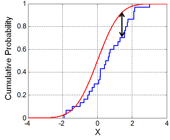A visualization of the Kolmogorov-Smirnov test statistic, taken from Wikipedia. The theorized CDF is shown in red, while the observed CDF is shown in blue. The maxiumum difference between the theorized CDF and the observed CDF is indicated with an arrow; this distance is the K-S statistic.

The Andersen-Darling test is similar, except that it doesn’t only consider the maximum value. Instead, it is defined as follows, where \(F(x)\) is the theorized cumulative distribution function (CDF), and \(F_n(x)\) is the observed CDF (because I’m ignoring the weight parameter, this is equivalent to the Cramér–von Mises statistic):

$$A^{2}=n\int_{-\infty }^{\infty }{\frac {(F_{n}(x)-F(x))^{2}}{F(x);(1-F(x))}},dF(x)$$

The Anderson-Darling test is especially notable for its ability to capture deviating ’tails’. Because our sample size is quite small and we are assessing fit to the uniform distribution, however, I think these normally-valuable properties of the Anderson-Darling test are less relevant to our context. Instead, we’ll opt for the simpler—albeit less powerful—K-S test.

Kolmogorov-Smirnov in Practice

Typically, when using the K-S test with a continuous theorized CDF, you can compare results against already-published critical values: values of \(D_n\) (the K-S test result) that indicate a certain confidence in the distribution’s fit. Unfortunately, our theorized distribution is a discrete uniform distribution; there are only ten digits, and therefore only ten possible values. Fortunately, we can determine an appropriate K-S test statistic threshold through simulations.⁶

We will determine our thresholds by generating thousands of sample observations by sampling the true distribution and calculating the K-S test statistic for each.⁷ The \(p\)-value parameter captures the probability that the generated threshold will falsely filter out observations that were drawn from the theorized distribution. For example, using a \(p\)-value of 0.2 to calculate the threshold (roughly) means that we will erroneously exclude 20% of observations that are drawn from the uniform distribution — but this trade-off between false-negatives and false-positives is necessary, and 0.2 is where we draw the line on the website.⁸

/* Function: ksStatTheshold
 * ------------------------
 * Calculate the K-S statistic value that,
 * if used as a threshold for
 * determining fit, would only exclude true
 * fits with probability `pVal`.
 */
function ksStatTheshold(pVal, n, sampleFunc, cdf) {
    const N_TRIALS = 10000;

    // Run many simulations
    let results = [];
    for(let i = 0; i < N_TRIALS; i++) {
        let sample = Array.from({length: n}, sampleFunc);
        let ksStat = kolmogorovSmirnov(sample, cdf);
        results.push(ksStat);
    }

    // Find the K-S test value that would only exclude
    // `pVal` of results. 
    results.sort((a, b) => a - b);
    return results[Math.floor((1 - pVal) * results.length)];
}

Using the power of simulation, we now have a probabilistically-sound way to evaluate the raw digit frequency distributions! Interestingly, I believe the function defined above is actually the (simulated) CDF of the Kolgomorov distribution—a beautiful distribution that captures the probability of a random sample having a particular K-S test value.⁹ While a detailed explanation of the Kolmogorov distribution is beyond the scope of this project, it is too cool not to mention!

Distances Between Numbers

Another way we can potentially detect humanity is by assessing the distances between numbers. If the human enters a 1 and then a 6, the distance is 5; if they enter a 5 and then another 5, the distance is 0. The distances between humans’ inputs might not distribute the same way that ’truly’ random digits would. For example, humans might avoid entering the same number twice — or at least they might do it at a statistically improbable rate.

We can assess adherence to the expected distribution the same way we did for the raw distribution. We just have one challenge: we need to figure out the expected distribution of the distances!

We can think of distance as a random variable \(D\) that is the absolute value of the difference between two discrete uniform random variables, \(U_1 \sim \text{Uni}(0, 9)\) and \(U_2 \sim \text{Uni}(0, 9)\):

$$D = |U_2 - U_1|$$

Unlike the expected distribution of the raw numbers (which was uniform), this distribution is less obvious. We can derive the probability mass function and use that to derive a cumulative distribution function, which we can then hand to our Kolmogorov-Smirnov function:

$$P(D = x) = P(|U_2 - U_1| = x)$$

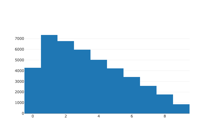The empirical distance PMF, obtained through simulations.

First let’s solve the non-absolute form; that is, instead of looking for the probability of particular distances, we instead look for the probability of particular differences. The maximum possible difference is 9 (\(U_1 = 0, U_2 = 9\)), and the minimum possible difference is -9 (\(U_1 = 9, U_2 = 0\)). We can use this PMF later on to calculate the ‘original’ PMF.

$$P_{\text{diff}}(x) = P(U_2 - U_1 = x) = \sum_{n = 0}^{9} P(U_2 = n) * P(U_1 = n - x)$$

Because \(U_1\) and \(U_2\) are discrete uniform random variables (with a range of 0 and 9, inclusive), their PMF is:

$$P(U = x) = \begin{cases} 0 & x < 0 \\ \frac{1}{10} & 0 \leq x \leq 9 \\ 0 & 9 < x \end{cases}$$

We now have everything we need to calculate the full PMF of \(D\):

$$P(D = x) = \begin{cases} 0 & x < 0 \\ P(D_1 = D_2) = \frac{1}{10} & 0 = x \\ P_\text{diff}(x) + P_\text{diff}(-x) & 0 < x \leq 9 \\ 0 & 9 < x \end{cases} $$

We can then plot this theorized PMF, revealing the original empirical PMF from above:

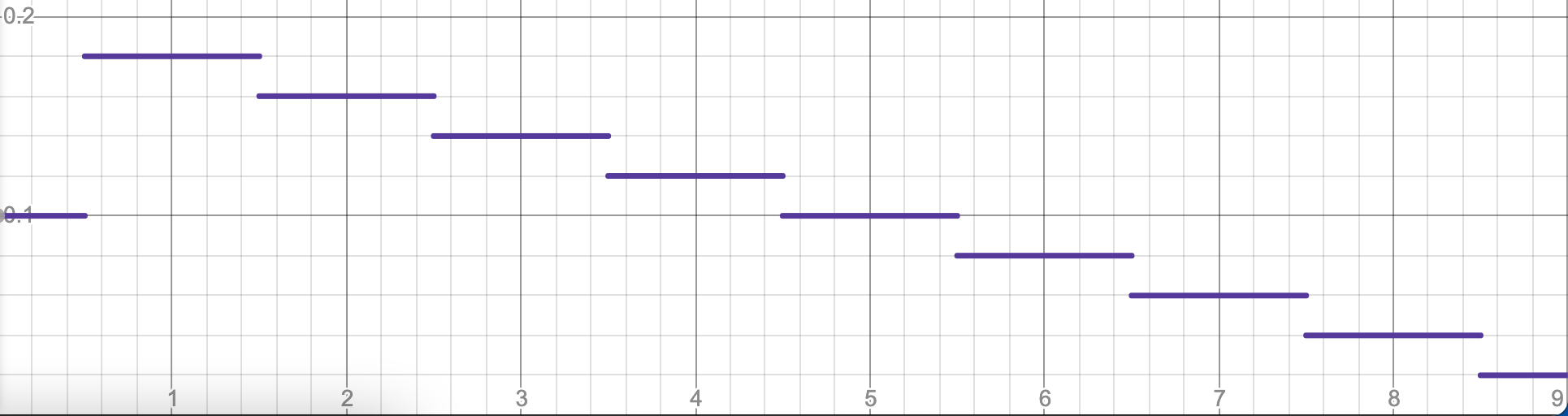The theorized PMF of the distance distribution.

Wonderful! We now have the PMF of our distance distribution. Because this is a discrete distribution, the CDF—we’ll call it \(F(x)\)—is as simple as a sum:

$$F(x) = \sum_{n=0}^{x} P(D = x)$$

We can now use the same technique as before to calculate our K-S test threshold.

The Website Itself

When visitors navigate to the Robot Club website, a friendly but firm robot bouncer greets them (see the image below). To continue, the visitor must enter 50 digits using their keypad.¹⁰ If the K-S test statistic for both the raw digit frequencies and the digit distances is below the threshold values, they are allowed entry.

Of course, the best way to experience the website is by visiting it yourself. Still, here are a few key highlights of the website. Note that I took these screenshots after an earnest effort to produce genuinely random numbers!

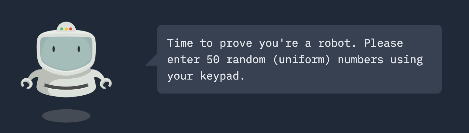The Robot Club’s bouncer, well known for its entropy evaluation skills. The robot graphic itself was made by Jessica Biggs on CodePen.

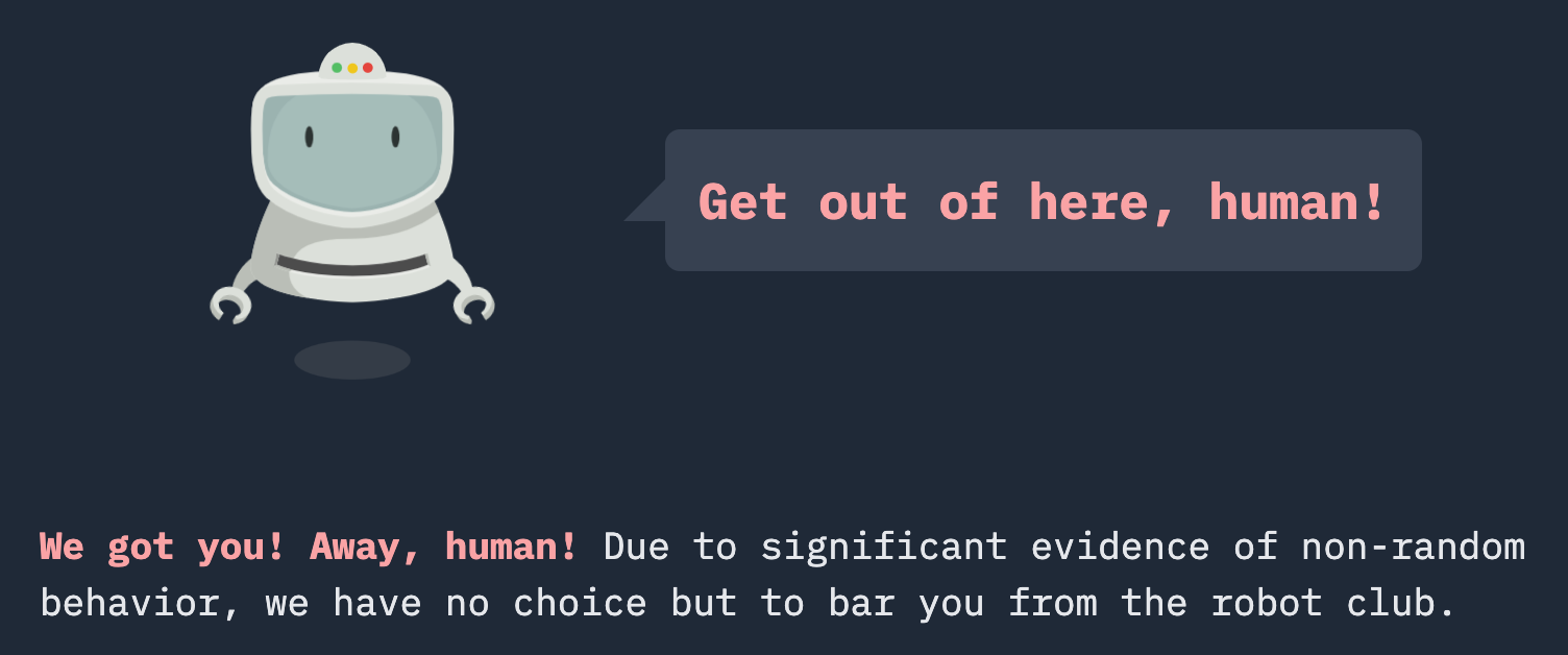The bouncer blocking me from the club; after all, I’m human!

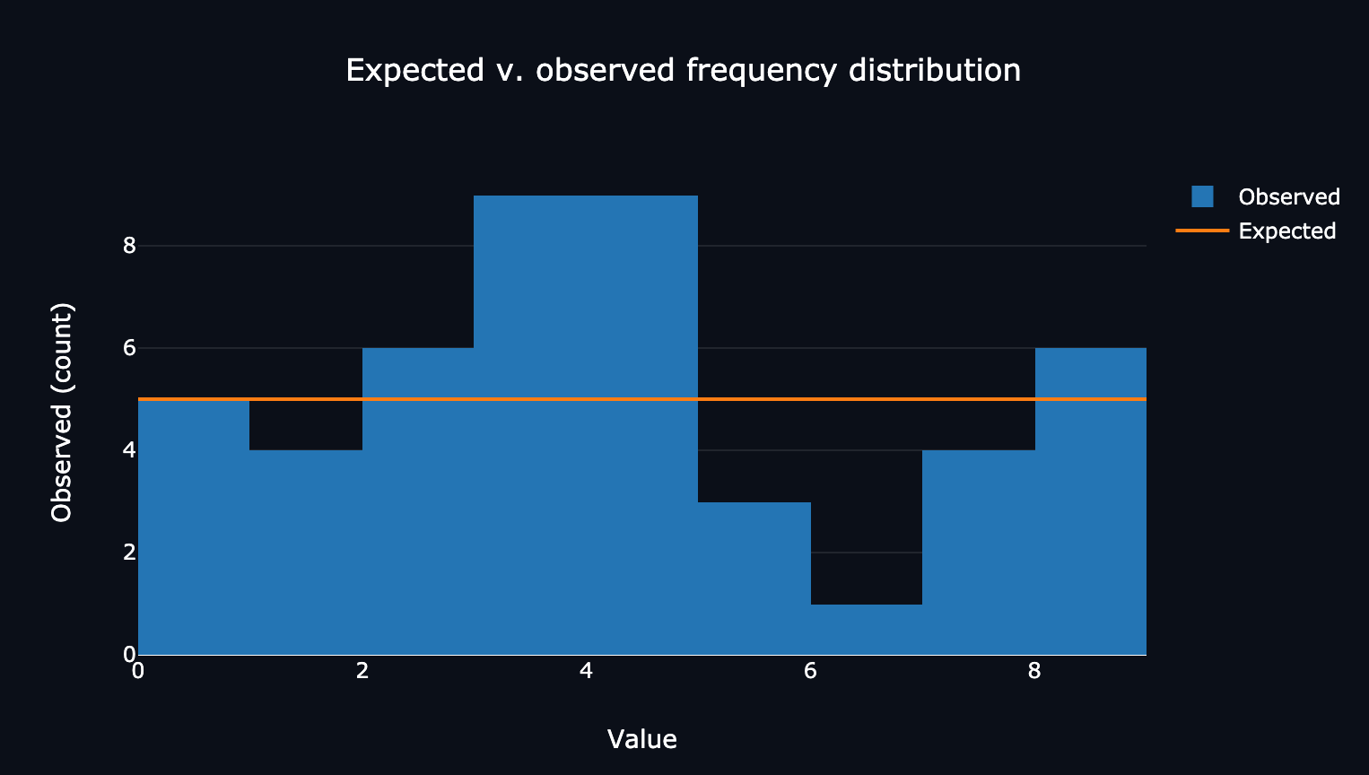The website’s breakdown of my digits’ frequencies compared to the expected values.

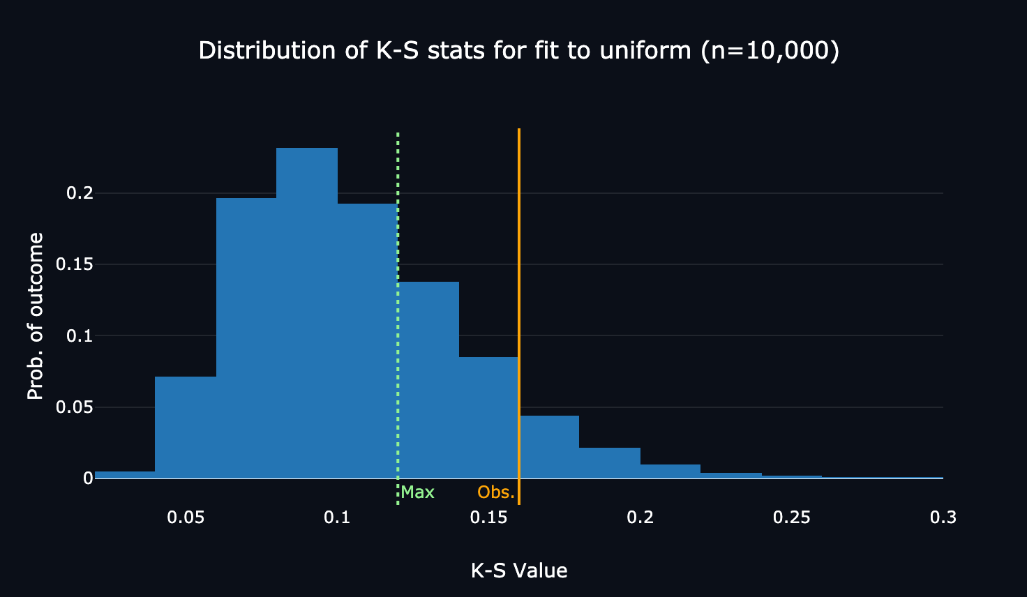The website’s visualization of the distribution of simulated true K-S test values for the frequency distribution, annotated with the maximum threshold and my score.

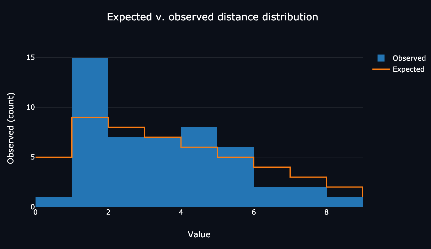The website’s breakdown of my digits’ distances compared to the expected values.

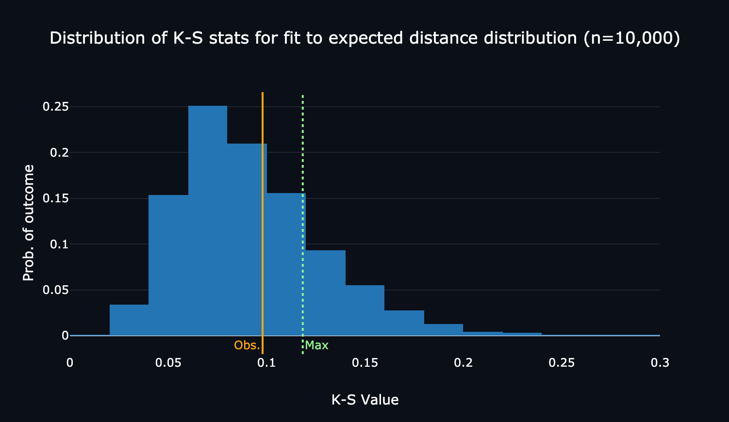The website’s visualization of the distribution of simulated true K-S test values for the distance distribution, annotated with the maximum threshold and my score. Here, I was below the maxiumum threshold!

On Thresholds and Error Rates

The website denies entry to the club if the K-S test statistic for either distribution is more extreme than 80% of the simulated samples (which were, in fact, drawn genuinely randomly). 80% is quite a low threshold for exclusion; assuming that the K-S test statistics for raw frequencies and distances are independent, then the club would exclude robots with probability \(1 - 0.8^2 = 0.36\) — an absolutely unacceptable false-negative rate. Still, in my experience (and in testing the website on friends) it does relatively well detecting humans: when I try to fool it, I get through about half the time. (A robot, meanwhile, makes it through around 64% of the time.) And none of my friends have gotten in on their first try.

While I wish I could compute the exact probability of the website letting a human in, doing so would require collecting loads of experimental data. I do think this could make for a great Mechanical Turk study, but that would require money and a more robust survey instrument — two things I don’t currently have and am not in a position to make. For now, my crude ‘anecdata’ will have to do.

The Future of the Robot Club

While the Robot Club’s entry assessment makes for a fun and educational probabilistic analysis, it is not as effective as it could be. With a false negative rate of 36%, more than a third of robots are denied entry! Furthermore, some simple digit patterns—such as 0, 9, 1, 8, 2, 7...—reliably ‘fool’ the bouncer into thinking the visitor is a robot. A more accurate way to assess signals of humanity in digits might be to train some kind of neural network on large samples of randomly-produced and human-produced digits. Neural networks, after all, are essentially pattern recognition machines.¹¹ This would require human training data, however, which I don’t have.

I also want to acknowledge the irony in assessing randomness by looking at predictability. While this of course makes sense after taking CS109—it’s the law of large numbers, after all—it is a bit counter-intuitive on its face.

Still, even with all these caveats, the Robot Club’s assessment system makes for a fun and educational probabilistic analysis. I certainly learned a lot. I hope you enjoyed your visit to the Robot Club — if you were able to get in, that is!

Endnotes